Im Zuge der diesjährigen Open Source Monitoring Conference durfte ich mit Timeseries & Analysis with Graphite and Grafana einen der Workshops am Vortag der eigentlichen Konferenz halten. Wie man dem Titel unschwer entnehmen kann spielte dabei auch Grafana eine besondere Rolle. Grafana ist vielen als schöneres Dashboard für Graphite bekannt und unterstützt mit Elasticsearch, CloudWatch, InfluxDB, OpenTSDB, Prometheus, MySQL als auch Postgres in der aktuellen Version 4.6.2 allerdings noch eine ganze Reihe weiterer Datensourcen nativ. Zusätzlich können diese herkömmlichen Datensourcen auch noch durch Community Plugins ergänzt werden.
Ganz besonders hilfreich ist es wenn man die Informationen aus verschiedenen Datensourcen miteinander vereint. So lassen sich beispielsweise Zusammenhänge besser erkennen und Rückschlüsse auf bestimmte Ereignisse ziehen, die ansonsten vielleicht unentdeckt blieben. Metriken, die z.B. aus Graphite stammen, können bei Grafana nun durch sogenannte Annotations um zusätzliche Informationen angereichert werden. Neben Annotations aus den unterstützten Datensourcen können solche Events seit v4.6 übrigens auch direkt in der eigenen Grafana-Datenbank gespeichert werden, ob man das wiederum möchte ist allerdings eine ganz andere Frage…
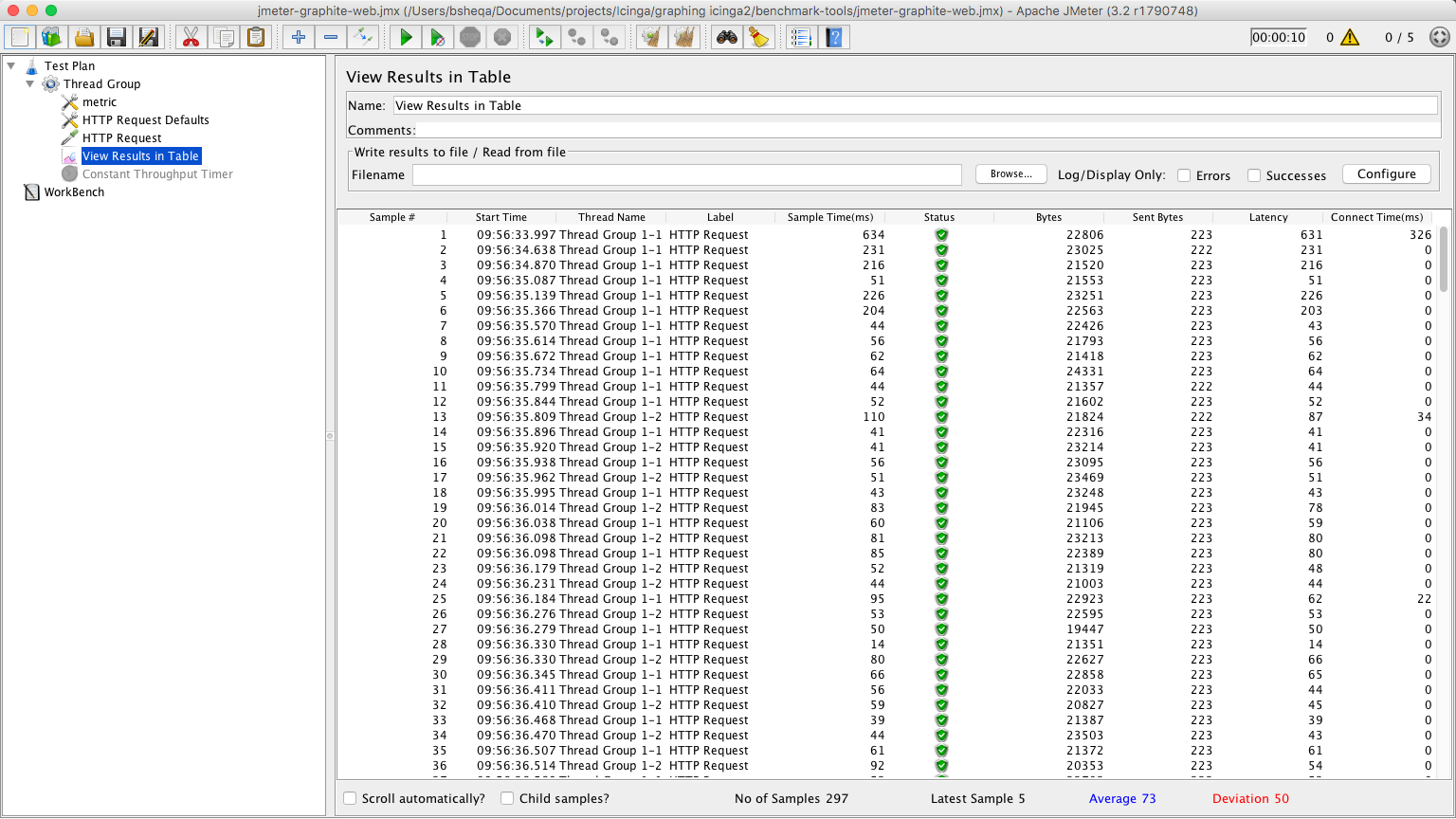
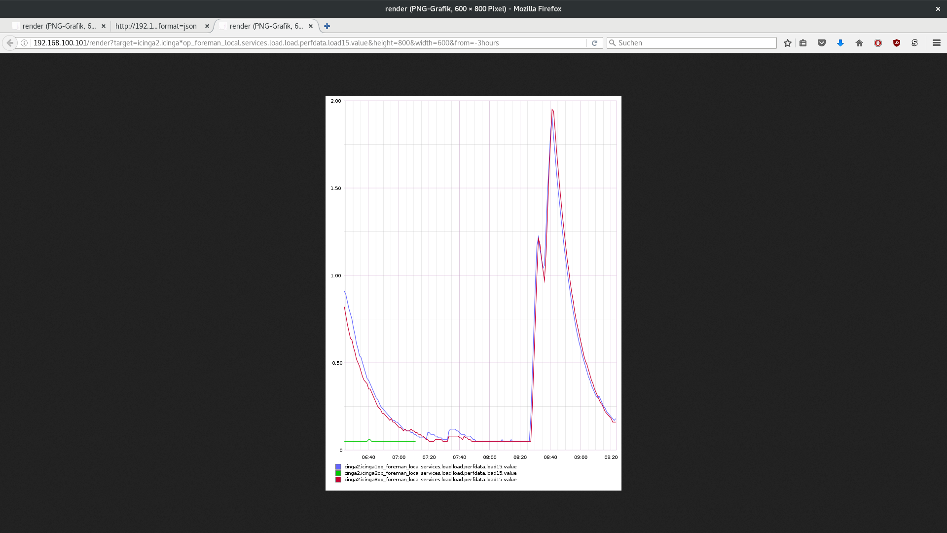
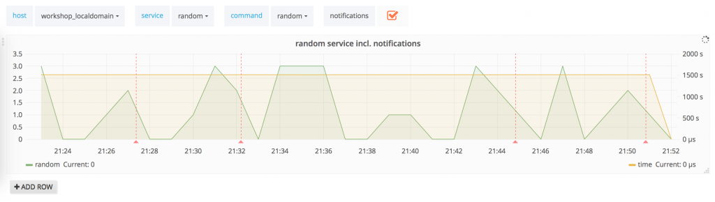
Als Praxisbeispiel habe ich für meinen Workshop im Rahmen der OSMC überraschenderweise Icinga gewählt. Hier ist es möglich über die Icinga 2 API verschiedene Daten wie Checkergebnisse, Statusänderungen, Benachrichtigungen, Bestätigungen, Kommentare oder auch Downtimes mit dem Icingabeat direkt an Elasticsearch oder wenn man möchte alternativ auch an Logstash zu senden. Über das Annotation-Feature von Grafana lassen sich so die Benachrichtigungen aus Icinga über die Elasticsearch Datasource passend zu den jeweiligen Statusänderungen der Host- oder Serivcechecks einblenden:
Wer dazu mehr erfahren möchte dem kann ich unsere Graphite + Grafana Schulung ans Herz legen, neben vielen anderen Themen werden dort auch Grafana und Annotations in aller Ausführlichkeit behandelt. Und wer’s nicht schafft, für den findet sich vielleicht der ein oder andere passende Workshop im Rahmen unserer Konferenzen.
NETWAYS Blog
Benchmarking Graphite
Before using Graphite in production, you should be aware of how much load it can handle. There is nothing worse than finding out your carefully planned and build setup is not good enough. If you are already using Graphite, you might want to know the facts of your current setup. Knowing the limits of a setup helps you to react on future requirements. Benchmarking is essential if you really want to know how many metrics you can send and how many requests you can make. To find this out, there are some tools out there that help you to run benchmarks.
Requirements
The most important thing you need when starting to benchmark Graphite is time. A typical Graphite stack has 3 – 4 different components. You need plenty of time to properly find out how much load each of them can handle and even more to decide which settings you may want to tweak.
Haggar
Haggar is a tool to simulate plenty of agents that send generated metrics to the receiving endpoint of a Graphite stack (carbon-cache
, carbon-relay
, go-carbon
, etc…). The amount of agents and metrics is configurable, as well as the intervals. Even though Haggar does not consume much resources, you should start it on a separate machine.
Haggar is written in go and installed with the go get
command. Ensure that Go (>= v1.8) is installed and working before installing Haggar.
Installing Haggar
go get github.com/gorsuch/haggar
You’ll find the binary in your GOPATH
that you have set during the installation of Go previously.
Running Haggar:
$GOPATH/bin/haggar -agents=100 -carbon=graphite-server.example.com:2003 -flush-interval=10s -metrics=1000
Each agent will send 1000
metrics every 10
seconds to graphite-server.example.com
on port 2003
. The metrics are prefixed with haggar.
by default. The more agents and metrics you send, the more write operations your Graphite server will perform.
Example output of Haggar:
root@graphite-server:/opt/graphite# /root/go/bin/haggar -agents=100 -carbon=graphite-server.example.com:2003 -flush-interval=10s -metrics=1000 2017/09/21 09:33:30 master: pid 16253 2017/09/21 09:33:30 agent 0: launched 2017/09/21 09:33:42 agent 1: launched 2017/09/21 09:33:46 agent 2: launched 2017/09/21 09:34:00 agent 0: flushed 1000 metrics 2017/09/21 09:34:02 agent 1: flushed 1000 metrics 2017/09/21 09:34:06 agent 2: flushed 1000 metrics
Testing the write performance is a good starting point, but it’s not the whole truth. In a production environment data is not only written but also read. For example by users staring at dashboards all day long. So reading the data is as much important as writing it because it also produces load on a server. This is where JMeter comes into play.
JMeter
Apache JMeter usually is used to test the performance of web applications. It has many options to simulate requests against a web server. JMeter can also be used to simulate requests against Graphite-Web. You should do this simultaneously while Haggar is sending data, so you have the “complete” simulation.
The easiest way to configure JMeter is the graphical interface. Running test plans is recommended on the command line, though. Here’s an example how I set up JMeter to run requests against Graphite-Web:
- Add a
Thread Group
to theTest Plan
- Set the Number of Threads (eg.
5
) - Set the loop count to
Forever
- Set the Number of Threads (eg.
- Add a
Random Variable
to theThread Group
- Name the variable
metric
- Set the minimum to
1
- Set the maximum to
1000
- Set `Per Thread` to
true
- Name the variable
- Add another
Random Variable
to theThread Group
- Name the variable
agent
- Set the minimum to
1
- Set the maximum to
100
- Set
Per Thread
totrue
- Name the variable
Haggar uses numbers to name it’s metrics. With these variables we can create dynamic requests.
- Add a
HTTP Request Defaults
to theThread Group
- Set the server name or IP where your Graphite-Web is running (eg.
graphite-server.example.com
) - Add the path
/render
to access the rendering API of Graphite-Web - Add some parameters to the URL, examples:
- width:
586
- height:
308
- from:
-30min
- format:
png
- target:
haggar.agent.${agent}.metrics.${metric}
- width:
- Set the server name or IP where your Graphite-Web is running (eg.
The most important part about the request defaults is the target
parameter.
- Add a
HTTP Request
to theThread Group
- Set the request method to
GET
- Set the request path to
/render
- Set the request method to
- Add a
View Results in Table
to theThread Group
The results table shows details of each request. On the bottom there is an overview of the count of all samples, the average time and deviation. Optionally you can also add a Constant Throughput Timer
to the Thread Group
to limit the requests per minute.
If everything is working fine, you can now start the test plan and it should fire lots of requests against your Graphite-Web. For verification, you should also look into the access logs, just to make sure.
At this point your Graphite server is being hit by Haggar and JMeter at the same time. Change the settings to find out at which point your server goes down.
Interpretation
Obviously, killing your Graphite server is not the point of running benchmarks. What you actually want to know is, how each component behaves with certain amounts of load. The good thing is, every Graphite component writes metrics about itself. This way you get insights about how many queries are running, how the cache is behaving and many more.
I usually create separate dashboards to get the information. For general information, I use collectd to monitor the following data:
Load
,CPU
,Processes
,I/O Bytes
,Disk Time
,I/O Operations
,Pending I/O Operations
,Memory
The other dashboards depend on the components I am using. For carbon-cache
the following metrics are very interesting:
Metrics Received
,Cache Queues
,Cache Size
,Update Operations
,Points per Update
,Average Update Time
,Queries
,Creates
,Dropped Creates
,CPU Usage
,Memory Usage
For carbon-relay
you need to monitor at least the following graphs:
Metrics Received
,Metrics Send
,Max Queue Length
,Attempted Relays
,CPU Usage
,Memory Usage
All other Graphite alternatives like go-carbon
or carbon-c-relay
also write metrics about themselves. If you are using them instead of the default Graphite stack, you can create dashboards for them as well.
Observing the behaviour during a benchmark is the most crucial part of it. It is important to let the benchmark do its thing for a while before starting to draw conclusions. Most of the tests will peak at the start and then calm after a while. That’s why you need a lot of time when benchmarking Graphite, every test you make will take its own time.
Performance Tweaks
Most setups can be tuned to handle more metrics than usual. This performance gain usually comes with a loss of data integrity. To increase the number of handled metrics per minute the amount of I/Ops must be reduced.
This can be done by forcing the writer (eg. carbon-cache
) to keep more metrics in the memory and write many data points per whisper update operation. With the default carbon-cache
this can be achieved by setting MAX_UPDATES_PER_SECOND
to a lower value than the possible I/Ops of the server. Another approach is to let the kernel handle caching and allow it to combine write operations. The following settings define the behaviour of the kernel regarding dirty memory ratio.
vm.dirty_ratio
(eg.80
)vm.dirty_background_ratio
(eg.50
)vm.diry_expire_centisecs
(eg.60000)
Increasing the default values will lead to more data points in the memory and multiple data points per write operation.
The downside of these techniques is that data will be lost on hardware failure. Also, stopping or restarting the daemon(s) will take much longer, since all the data needs to be flushed to disk first.
Revisited – Graphite-Web installation unter Debian 9
Erstmal wieso Revisited ?
Dies ist ein update meines älteren Blog Posts Blogpost 2016 welcher darauf einging das unter Debian 8.4 graphite-web wegen eines Fehlenden Eintrages in der Apache 2.4 Konfiguration nicht korrekt gestartet/aufgerufen werden konnte.
Es ist schon einige Zeit ins Land gegangen und ich habe weniger ein Auge darauf geworfen ob das weiterhin so Funktioniert.
Deshalb Revisited.
Here we Go again !
Ich gehe in diesem Fall von einer Debian Version der Nummer 9 aus und werde wie bei dem alten Blogpost. In der Grundannahme mal davon ausgehen das alles Funktioniert wie es soll:
Also hier die folgenden installationschritte:
#> apt-get install apache2 libapache2-mod-wsgi python-django python-django-tagging fontconfig python-tz python-pip python-dev python-twisted python-cairo
#> pip install carbon whisper graphite-web
#> pip install --upgrade twisted
#> cp /opt/graphite/conf/carbon.conf.example /opt/graphite/conf/carbon.conf
#> cp /opt/graphite/conf/storage-schemas.conf.example /opt/graphite/conf/storage-schemas.conf
#> /opt/graphite/bin/carbon-cache.py start
#> /opt/graphite/bin/carbon-cache.py status
#> cp /opt/graphite/examples/example-graphite-vhost.conf /etc/apache2/sites-available/graphite.conf
#> cp /opt/graphite/conf/graphite.wsgi.example /opt/graphite/conf/graphite.wsgi
#> cp /opt/graphite/webapp/graphite/local_settings.py.example \ /opt/graphite/webapp/graphite/local_settings.py
#> python /opt/graphite/webapp/graphite/manage.py syncdb
#> chown www-data. -R /opt/graphite/storage
#> a2dissite 000-default
#> a2ensite graphite
#> a2enmod wsgi
#> service apache2 restart
#> chmod +x /etc/init.d/carbon-cache // Damit 'carbon-cache.py start' mit Systemstart erfolgt
Ergebnis davon ist -> Nichts funktioniert.
Back to the Roots
Ab hier kommt der Weg graphite-web auf einem Debian 9 (Stretch) in Betrieb zu nehmen.
Ausgangspunkt ist ein frisch installiertes Debian 9.
#> apt-get install vim -y
#> vim /etc/apt/sources.list
Wir müssen die Sources auf die Jessie Repositories setzen da zum Zeitpunkt dieses Blogposts die graphite-web Pakete nicht abrufbar sind.
Daher fügen wir folgendes hinzu in der sources.list
deb http://httpredir.debian.org/debian jessie main
Gefolgt von einem frischem #> apt-get update -y
.
Nun installieren wir den großteil der Pakete welche wir benötigen.
#> apt-get install graphite-web graphite-carbon mysql-server python-mysqldb python-pymysql apache2 libapache2-mod-wsgi apt-transport-https ssl-cert python-pip -y
Es folgen ca. 300MB an Daten.
Daraufhin stürzen wir uns direkt auf die Konfig.
Wir fangen an folgende Datei zu editieren.
#> vim /etc/graphite/local_settings.py
Darin ändern wir folgende Settings Sinnvoll in etwas was wir für unsere Installation benötigen.
Also SECRET_KEY, TIME_ZONE & ALLOWED_HOSTS setzen.
Danach muss in der folgenden Datei ein „true“ gesetzt werden damit graphite & carbon gemeinsam starten.
#> vim /etc/default/graphite-carbon
Nun kommt der trickreichste Part wir sind leider dazu genötigt eine alte django Version zu installieren.
#> pip install "django==1.4"
Damit haben wir die Grundlage womit wir das folgende Kommando erfolgreich absetzen können.
#> graphite-manage syncdb
#> Kundenverbesserung: Danke an bbtronic!
#> graphite-manage migrate --run-syncdb
#> chown _graphite. /var/lib/graphite/graphite.db
HINWEIS ! Dies setzt erst mal die voreingestellte sqlitedb in Gang.
Wenn eine andere DB verwendet werden soll dann sollte dies bitte in der „local_settings.py“ vorgenommen werden.
Wir sind fast am Ziel ein funktionierendes graphite-web zu haben.
Es fehlt nur etwas Apache2 Magie.
#>a2dissite 000-default.conf
#>cp /usr/share/graphite-web/apache2-graphite.conf /etc/apache2/sites-available/
#> a2ensite apache2-graphite.conf
#> systemctl restart apache2
Voilà !
Es sollte nun auf dem Host System das graphite-web aufrufbar sein.
Danke für die Aufmerksamkeit !
Addenum nicht Sichtbare Kommentare von Kunden:
# Oliver: Ich bekam leider den Fehler:
twisted.python.usage.UsageError: Unknown command: carbon-cache
Hier hat dies geholfen:
mv /usr/local/lib/python2.7/dist-packages/twisted /usr/local/lib/python2.7/dist-packages/twisted2
Hier half mir ein downgrade:
python -m pip install ‘django-tagging<0.4'
Das hatte ich auch, habe es mit upgrade auf django 1.5 beseitigen können:
python -m pip install django==1.5
Vinc:
hallo David
nach dem ich die Installation bei back to the roots gestartet habe, klappte es. Wobei ein paar Infos unter Also SECRET_KEY, TIME_ZONE & ALLOWED_HOSTS wäre wohl noch nützlich.
Aber trotzdem – klappt es nicht – die “bilder” erscheinen nicht wie wenn der Pfad falsch ist.
gruss
vinc
Graphite Reporting mit der Render-API
Vor kurzem durfte ich mich damit beschäftigen, wie man schnell und halbwegs vernünftig eine Art Reporting für Performance-Daten für Icinga 2 umsetzen kann. Um solche Daten entsprechend aufzubereiten bedarf es weiterer Open-Source-Software. Meiner Meinung nach eignet sich Graphite hierzu am besten. Ich möchte heute einen kurzen Einblick in die Möglichkeiten geben.
Graphite ist ein Werkzeug, welches aus drei Komponenten besteht: Carbon-Cache als Datensammler, Whisper als Storage-Backend und Graphite-Web um die Graphen visuell und als API bereitzustellen. Icinga 2 schreibt die Performance-Daten mit dem „graphite“-Feature direkt an den Carbon-Cache-TCP-Socket. Welche Möglichkeiten habe ich als Anwender nun, diese historischen Daten für meine Zwecke in Reporting zu verwenden?
Eigentlich ganz einfach: Graphite liefert eine eigene Render-API. Diese bietet die Möglichkeit, die Daten als Graph, csv , json, pdf und einige weitere Formate zu generieren. Der Anwender kann diese Daten als REST-API Aufruf im Browser oder beispielsweise curl in der Shell abholen. Dabei können verschieden Metriken und Aggregationen auf Graphen angewandt und unterschiedliche Werte gebündelt abgerufen werden.
Wie fange ich an?
Generell wird die URL wie folgt aufgebaut:
target=icinga2..services.*.*.perfdata.*.value
Im gezeigten Beispiel kann man für die „target“-Metriken auch Wildcards verwenden, um etwa mehrere Services gleichzeitig abzufragen. Dies entspricht dem Dateipfad im Whisper-Backend. Man kann allerdings auch Listen oder Arrays angeben, um gezielt bestimmte Werte abzufragen.
Es gibt unterschiedliche Möglichkeiten, die Daten für die entsprechenden Ausgaben weiterzuverarbeiten. Die wohl wichtigsten sind &from für die Zeit und &format für die Formatierung der Daten.
Metrik „Baum“
Um die Werte für die CPU-Load abzufragen, muss der entsprechende Service in Icinga 2 definiert sein und Performance-Daten nach Graphite schreiben. Im Screenshot sieht man im Baum „services“ – „load“, letzterer stellt den Service-Namen dar. Der Sub-Knoten „load“ liefert die Information, dass hier das „load“ CheckCommand verwendet wurde. Tip an dieser Stelle: Lässt sich etwa für Dashboard-Templates als eindeutiger Schlüssel verwenden in Grafana.
Performance-Daten liefern zum einen „perfdata“, worin einzelne Metriken mit ihrem Namen abgelegt werden, etwa „load1“ und darunter „value“ als Wert und Thresholds, etwa „crit“ und „warn“, sofern definiert. Zusätzlich können auch Metadaten von Icinga 2 geschrieben werden, die man aber explizit in der Konfiguration einschalten muss („metadata“).
Einzelne Metrik abfragen
Im folgenden interessiert uns aber lediglich der Wert der Metrik „load1“ als einzelner Wert. Um eine ordentliche Ausgangsbasis zu erhalten, wählen wir den Zeitraum der letzten 3 Stunden. Tip: Es sind relative und absolute Zeitangaben möglich.
http://192.168.100.101/render?target=icinga2.icinga3op_foreman_local.services.load.load.perfdata.load1.value&height=800&width=600&from=-3hours
Mehrere Metriken zusammenfassen
Man kann diese Abfrage auch erweitern, indem man mehrere Werte gleichzeitig abfrägt:
http://192.168.100.101/render?target=icinga2.icinga3op_foreman_local.services.load.load.perfdata.{load1,load15,load5}.value&height=800&width=600&from=-3hours
Mehrere Hosts mit der gleichen Metrik abfragen
Eine Abfrage mit verschiedenen Servern für „load15“ als Metrik könnte so aussehen:
http://192.168.100.101/render?target=icinga2.icinga*op_foreman_local.services.load.load.perfdata.load15.value&height=800&width=600&from=-3hours
Formatierung
Die Darstellung der Daten setzt immer eine &height und eine &width als Parameter voraus. Es ist auch möglich hier Tortendiagramme mit verschiedenen Funktionen für Mittelwerte und Summen aufzurufen.
Man kann die erhaltenen Daten auch als CSV-Werte formatieren und dann beispielsweise mit curl abspeichern. Alternativ kann man sich diese Werte auch direkt im Browser anzeigen lassen.
[root@icinga1op ~]# curl 'http://192.168.100.101/render/?target=icinga2.icinga3op_foreman_local.services.load.load.perfdata.load5.value&from=-3hours&format=csv' icinga2.icinga3op_foreman_local.services.load.load.perfdata.load5.value,2017-06-16 06:30:00,0.24 icinga2.icinga3op_foreman_local.services.load.load.perfdata.load5.value,2017-06-16 06:31:00,0.21 icinga2.icinga3op_foreman_local.services.load.load.perfdata.load5.value,2017-06-16 06:32:00,0.17 icinga2.icinga3op_foreman_local.services.load.load.perfdata.load5.value,2017-06-16 06:33:00,0.15 icinga2.icinga3op_foreman_local.services.load.load.perfdata.load5.value,2017-06-16 06:34:00,0.16 icinga2.icinga3op_foreman_local.services.load.load.perfdata.load5.value,2017-06-16 06:35:00,0.13 icinga2.icinga3op_foreman_local.services.load.load.perfdata.load5.value,2017-06-16 06:36:00,0.12 ....
Wie bereits erwähnt lassen sich die Daten auch im JSON-Format anzeigen. Dies kann wieder über den Browser oder mittels curl erfolgen.
Das folgende Beispiel rendert alle erhaltenen Datenpunkte als JSON-Format:
[root@icinga1op ~]# curl 'http://192.168.100.101/render/?target=icinga2.icinga3op_foreman_local.services.load.load.perfdata.load5.value&from=-3hours&format=json' [{"target": "icinga2.icinga3op_foreman_local.services.load.load.perfdata.load5.value", "datapoints": [[0.13, 1497595140], [0.11, 1497595200], [0.15, 1497595260], [0.13, 1497595320], [0.1, 1497595380], [0.08, 1497595440], [0.07, 1497595500], [0.06, 1497595560], [0.06, 1497595620], [0.05, 1497595680], [0.04, 1497595740], [0.07, 1497595800], [0.05, 1497595860], [0.04, 1497595920], [0.05, 1497595980], [0.04, 1497596040], [0.08, 1497596100], [0.06, 1497596160], [0.07, 1497596220], [0.06, 1497596280], [0.06, 1497596340], [0.05, 1497596400], [0.04, 1497596460], [0.04, 1497596520], [0.03, 1497596580], [0.05, 1497596640], [0.04, 1497596700], [0.05, 1497596760], [0.04, 1497596820], [0.09, 1497596880], [0.07, 1497596940], [0.06, 1497597000], [0.06, 1497597060], [0.05, 1497597120], [0.04, 1497597180], [0.04, 1497597240], [0.03, 1497597300], [0.02, 1497597360], [0.02, 1497597420], [0.01, 1497597480], [0.01, 1497597540], [0.01, 1497597600], [0.01, 1497597660], [0.01, 1497597720], [0.01, 1497597780], [0.07, 1497597840], [0.06, 1497597900], [0.07, 1497597960], [0.08, 1497598020], [0.07, 1497598080], [0.06, 1497598140], [0.04, 1497598200], [0.04, 1497598260], [0.03, 1497598320], [0.14, 1497598380], [0.14, 1497598440], [0.13, 1497598500], [0.12, 1497598560], [0.1, 1497598620], [0.09, 1497598680], [0.09, 1497598740], [0.07, 1497598800], [0.06, 1497598860], [0.07, 1497598920], [0.1, 1497598980], [0.1, 1497599040], [0.08, 1497599100], [0.06, 1497599160], [0.05, 1497599220], [0.04, 1497599280], [0.04, 1497599340], [0.03, 1497599400], [0.02, 1497599460], [0.05, 1497599520], [0.04, 1497599580], [0.03, 1497599640], [0.03, 1497599700], [0.04, 1497599760], [0.05, 1497599820], [0.04, 1497599880], [0.04, 1497599940], [0.04, 1497600000], [0.04, 1497600060], [0.03, 1497600120], [0.03, 1497600180], [0.02, 1497600240], [0.01, 1497600300], [0.01, 1497600360], [0.01, 1497600420], [0.04, 1497600480], [0.04, 1497600540], [0.03, 1497600600], [0.03, 1497600660], [0.02, 1497600720], [0.04, 1497600780], [0.04, 1497600840], [0.03, 1497600900], [0.03, 1497600960], [0.02, 1497601020], [0.01, 1497601080], [0.01, 1497601140], [0.01, 1497601200], [0.01, 1497601260], [0.01, 1497601320], [0.01, 1497601380], [0.01, 1497601440], [0.01, 1497601500], [0.01, 1497601560], [0.01, 1497601620], [0.63, 1497601680], [1.29, 1497601740], [1.87, 1497601800], [2.4, 1497601860], [2.74, 1497601920], [2.36, 1497601980], [1.93, 1497602040], [1.58, 1497602100], [1.29, 1497602160], [1.7, 1497602220], [2.26, 1497602280], [2.77, 1497602340], [3.1, 1497602400], [3.37, 1497602460], [3.09, 1497602520], [2.56, 1497602580], [2.09, 1497602640], [1.71, 1497602700], [1.4, 1497602760], [1.16, 1497602820], [0.95, 1497602880], [0.78, 1497602940], [0.63, 1497603000], [0.52, 1497603060], [0.42, 1497603120], [0.35, 1497603180], [0.28, 1497603240], [0.23, 1497603300], [0.19, 1497603360], [0.16, 1497603420], [0.13, 1497603480], [0.12, 1497603540], [0.1, 1497603600], [0.08, 1497603660], [0.07, 1497603720], [0.05, 1497603780], [0.07, 1497603840], [0.06, 1497603900], [0.05, 1497603960], [0.04, 1497604020], [0.03, 1497604080], [0.03, 1497604140], [0.02, 1497604200], [0.02, 1497604260], [0.01, 1497604320], [0.01, 1497604380], [0.01, 1497604440], [0.01, 1497604500], [0.01, 1497604560], [0.01, 1497604620], [0.01, 1497604680], [0.01, 1497604740], [0.01, 1497604800], [0.01, 1497604860], [0.04, 1497604920], [0.05, 1497604980], [0.06, 1497605040], [0.08, 1497605100], [0.06, 1497605160], [0.07, 1497605220], [0.06, 1497605280], [0.04, 1497605340], [0.05, 1497605400], [0.04, 1497605460], [0.03, 1497605520], [0.03, 1497605580], [0.02, 1497605640], [0.02, 1497605700], [0.01, 1497605760], [0.01, 149760
Um die Daten leserlich in der Konsole aufzubereiten, empfiehlt es sich „python -m json.tool“ als Formatierungshilfe zu verwenden.
curl 'http://192.168.100.101/render/?target=icinga2.icinga3op_foreman_local.services.load.load.perfdata.load5.value&from=-3hours&format=json' | python -m json.tool
Um die JSON-Daten in der Console zu visualisieren kann man Zach Holman’s Spark verwenden:
[root@graphite ~]# curl 'http://192.168.100.101/render/?target=icinga2.icinga3op_foreman_local.services.load.load.perfdata.load5.value&from=-3hours&format=json' | python -mjson.tool | grep ',' | grep -v '\]' | spark % Total % Received % Xferd Average Speed Time Time Time Current Dload Upload Total Spent Left Speed 100 3695 0 3695 0 0 230k 0 --:--:-- --:--:-- --:--:-- 240k ▁▁▁▁▁▁▁▁▁▁▁▁▁▁▁▁▁▁▁▁▁▁▁▁▁▁▁▁▁▁▁▁▁▁▁▁▁▁▁▁▁▁▁▁▁▁▁▁▁▁▁▁▁▁▁▁▁▁▁▁▁▁▁▁▁▁▁▁▁▁▁▁▁▁▁▁▁▁▁▁▁▁▁▁▁▁▁▁▁▁▁▁▁▁▁▁▁▁▁▁▁▁▁▁▁▃▃▅▅▅▃▃▃▃▅▅███▅▅▃▃▃▁▁▁▁▁▁▁▁▁▁▁▁▁▁▁▁▁▁▁▁▁▁▁▁▁▁▁▁▁▁▁▁▁▁▁▁▁▁▁▁▁▁▁▁▁▁▁▁▁▁▁▁▁▁▁▁
Conclusio
Das war nur ein kleiner und rudimentärer Überblick was über die Render-API möglich ist. Jedoch bietet sie genügend Anregung um mehr mit Graphite, Icinga 2 und Metriken zu machen. Die Render-APi bietet zudem die Möglichkeit, programmatisch in Scripts darauf zuzugreifen. Mir hat es zumindest Lust auf mehr gemacht und ich denke, dass ich noch weitere Blogposts zu diesem Thema schreiben werde 🙂
Falls ihr nicht warten könnt, hier nochmal der Link zur Doku. Oder ihr schaut einfach mal bei uns in der Graphite-Schulung vorbei und lernt die Render-API am praktischen Beispiel kennen.
Monthly Snap May < GitLab CE, Icinga 2, NWS, OSDC, Ubuntu, Graphite, Puppet, SuiteCRM
In May, Achim started with GitLab CE, while Florian presented Vanilla.
Then, Lennart wrote the fifth part of his Icinga Best Practices and Isabel told us about the MultiTech MTD-H5-2.0.
Martin K. continued with external monitoring of websites and services with Icinga 2 while Julia gave a triple hurray to our OSDC-sponsors. Stefan G. gave an insight in his „Mission Loadbalancer Upgrade“ and Blerim tested Ruby applications with RSpec and WebMock.
Lennart published part 3 and 4 of „Icinga 2 – Automated Monitoring with Puppet„, Martin K. showed the benefits of our SuiteCRM Hosting while Marius G. told us the upcoming death of Ubuntu Unity.
May went on with the OSDC in Berlin and the reports from Isabel, Julia, Michi and Dirk.
Then Thomas Widhalm continued with the Carbon Relay for Graphite and Christian wrote about the Icinga 2 Satellite in NWS.
Towards the end of May, Christian announced some new webinars and Gabriel gave an insight in his work at NETWAYS!